Creating an Interactive Map

Objective

Now we will create our map, which has a dual objective: for a given year, our client wants to see the average pesticide concentration per region but also to identify the water treatment plants in which a non-compliant sample has been recorded during the year. By mousing over a plant, a user will be able to view the non-compliant pesticides detected by using the graphic that we previously produced.

Regional layer

Create a new spreadsheet and name it Regional map. Now let’s produce our map:

• Double-click latitude (dimension in dim_plant).
• Double-click longitude (dimension in dim_plant).
• Double-click concentration_moyenne (average concentration) (measure in facts_prelevements.csv).
• Right-click nom_region (name_region)(dimension in dim_plant) and select Rôle géographique (Geographical role) > NUTS Europe.
• Double-click nom_region.
• In the top right-hand corner of your work space, click Montre-moi (Show me) and choose the second style of map. Don’t do anything else and wait for the map to be generated.

Let’s return to a problem which should be one of your ongoing concerns: the properties associated with the additivity of measures. If you have a concentration of 0.05µg/L for two plants, this doesn’t mean that the concentration for all plants is 0.1µg/L! We need to calculate the average concentrations. At present, by default, Tableau calculates the sum of the average concentrations (SUM(concentration_moyenne)) per region. Consequently, if a region has more plants, it will have more samples, which will therefore increase its average concentrations.

• Remedy this problem by designating moyenne (average) as the aggregation function. Click the arrow on the right-hand side of the SUM(concentration_moyenne) field in the Repères (Locators) space and choose Mesure > Moyenne

Now let’s improve the key and the choice of color scale.

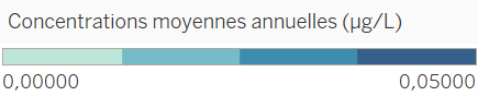
• Change the title of the key MOY(concentration_moyenne) to Concentrations moyennes annuelles (µg/L) (Average annual concentrations).
• Choose the option Modifier les couleurs (Change colors), select a échellonné en 4 étapes (4-level graduation) display, set the start at 0 and the end at 0.05.

Lastly, we want to filter the results per year. To do this:

• Move the annee (year) field (facts_samples attribute) into the Filtre (Filter) space and choose the year 2012, for example.
• Right-click the newly created field and choose Afficher le filtre (Display the filter).
• On the right-hand side of the new key, change the title to Année and then choose the option Valeur unique (liste déroulante) (Single value (scrollable list).

Superimposing the treatment plants

To display the plants superimposed on the map, you will need to create a double observation axis.

• In the Lignes (Rows) space, click latitude, and hold down the CTRL key while dragging and dropping the latitude attribute toward the right.
• Click the right-hand arrow of this new latitude attribute and select Axe double (Double axis). Wait while the calculations are completed and the map is updated.

Once the cursor has indicated that loading has finished, we can configure the display settings for our plants. To do this, start by selecting the latitude (2) tab in the Repères space. We are now in the right place to configure the double axis that we have just created.

• Delete the 2 attributes nom_region and AVG(concentration moyenne) shown in the tab
• Double-click code_station (plant code) (attribute of dim_station)
• Double-click respect_norme (compliance_standard) and then Couleur (Color) to assign green to Oui (Yes) and red to Non (No).

We need to be able to filter the treatment plants in order to display only those exceeding the levels set by the standard. To do this:

• Move the respect_norme attribute into the Filtres space and choose the Afficher le filtre (Display filter) option

Now perform a test with only one type of plant: compliant or non-compliant. What do you observe? We can see that plants displayed change, of course, but that the colors of the regions also change. This is due to the fact that the filter affects both maps - the plant map and the region map - and therefore skews the calculation of the average concentrations in the regions. Remove the respect_norme field from the Filtres space and from the Repères space for the latitude (2) tab.

We will need to create a calculated variable that will enable us to filter the plants on one of our views only. To do this:

• Click the Analyse (Analysis) menu and choose Créer un champ calculé (Create a calculated field).
• Name this field respect_norme_filtre (compliance_standard_filter) and add the following code to the window, which will assign the NULL value to compliant plants and the Hors-norme (Non-compliant) value to the others:

IF [compliance_standard]=='No' THEN 'Non-compliance standard' END

• Double-click the respect_norme_filtre field
• Rename the respect_norme_filtre key as Plants
• In this same key, right-click Null and choose the option Masquer (Hide)
• If necessary, choose red as the color for the Hors-norme values. To do this, click the Couleur button in the Latitude (2) space

Creating tooltips and synchronizing with the bar chart

To obtain contextual information by mousing over the regions and plants, we will create tooltips.

In the Repères space in the latitude tab, click the Infobulle (Tooltip) icon and cut and paste the following code into the window:

Region 	<nom_region>  
Annual average pesticide concentration  : <MOY(concentration_moyenne)> µg/L

For the tooltip on plants, we want to display a lot more information. We will need to make the attributes available for the tooltip. To do this, drag and drop each of the following attributes onto the tooltip icon in the latitude (2) tab:

• code_station (plant_code)
• nom_commune (name_municipality)
• nom_departement (name_department)
• nom_region (name_region)
• nom_sage (name_sage)
• annee (year)

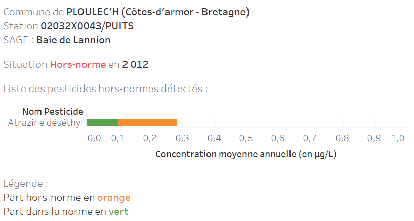
Finally, click the Infobulle icon and cut and paste the following code into the window (notice the line that begins with <Sheet, which enables the bar chart to be displayed in the tooltip, giving the list of pesticides tested as non-compliant by the treatment plant indicated by the cursor):

Municipality of <ATTR(name_municipality)> (<ATTR(name_department)> - <ATTR(name_region)>)
Plant <ATTR(plant_code)>
SAGE:	<ATTR(name_sage)>

non-compliant situation in <ATTR(year)>

List of non-compliant pesticides detected:

<Sheet name="tooltip:pesticides_plant" maxwidth="800" maxheight="400" filter="<ATTR(plant_code)>">

Key:
non-compliant proportion in orange
Compliant proportion in green

Experiment with formatting the tooltip (text highlighted in bold, colors, etc.) to imitate the image below:

To ensure that the bar chart takes account of the filter defined at the level of the interactive map, you need to configure it in Tableau.

• Go to the Filtres space.
• Right-click annee: 2012.
• Select Appliquer au feuilles de calculs > Feuilles de calculs sélectionnées. (Apply to spreadsheets > Selected spreadsheets)
• Check the box in front of tooltip:pesticides_plant.

To finish, change the title of the graphic to “Pesticide concentrations in groundwater and location of noncompliant plants” by right-clicking the title.

Overview of the final configuration

Back to main page